Self-Organizing Networks

I. Introduction

Constantly evolving mobile cellular systems are adding more and more services, especially for smartphones, so using these devices is increasingly essential. As of the fourth generation, in which 4G Long Term Evolution (LTE) technology began to offer high-speed connectivity, demand for user-generated traffic grew exponentially. Growth is being further accentuated with the introduction of fifth generation 5G NR – New Radio technology, which is not only faster than LTE but also enables even more applications. 5G and its verticals reach more users and different types of devices, which generates more traffic and takes cellular mobile networks to the next level in global communication. Cell phone operators increasingly require robustly capillarized infrastructure to offer services at the level of quality expected of them. This will need many more radio base stations and therefore higher operating costs. This scenario crucially requires Self-Organizing Networks to optimize systems with more automation and higher-level quality of service while lowering CAPEX (Capital Expenditure) and OPEX (Operational Expenditure).

II. What are SONs?

Self-Organizing Networks have evolved from conventional RAN (Radio Access Networks) and consist of a set of features designed to assist mobile network planning, configuration, management, optimization, and healing processes. SONs’ continuously automated operations reduce the need for human intervention during their activity while accelerating diagnostics and executing modifications depending on network behavior and operators’ purposes, in which everything has to be done efficiently in the functional context. These networks are characterized by three axes: self-configuration, self-optimization, and self-healing. Their architecture may be decentralized (Decentralized SON, or DSON), centralized (Centralized SON, C-SON) or hybrid (Hybrid SON, or H-SON) [1].

II.1. Centralized SON architecture

Centralized SON architecture operations are executed at network management level. Data for commands, requisitions, and parameter settings flow from the network’s management system to its elements, while metric and reporting data flow in the opposite direction. The main benefit of this architecture is that SON algorithms may factor in information from every part of the network. This means that all SON function parameters may be jointly optimized centrally so the network may more globally optimized, especially for functions that vary gradually. In addition, centralized solutions may be more robust at handling network instabilities caused by simultaneously operating SON functions with conflicting objectives; since all SON functions are centrally controlled, they can be easily coordinated without conflicts. Another advantage is that SON solutions from multiple vendors may be built in, since a functionality may be added at network management level rather than at network elements, where vendor-specific solutions are often required.

The main disadvantages of centralized SON architecture are longer response times, heavier backbone traffic, and the fact of their having one centralized fault point. Longer response time limits a network’s ability to speedily adapt to changes and may even cause instabilities. There is more backbone traffic because measurement data must be sent from network elements to the network management system and instructions must be sent in the opposite direction. Traffic will get heavier as more network elements are added. If there are many pico/femto-cells, traffic can be very heavy. Moreover much more centralized processing power will be required.

II.2. Distributed (decentralized) SON architecture

Distributed SON architecture operations are run on network elements, which in turn exchange SON-related messages directly with each other. This architecture can make SON functions much more dynamic than centralized SON solutions, and the solution scales very well as the number of elements in a network increases.

The main disadvantages are that the sum of all optimizations made at network element level does not necessarily result in optimal operation for the network as a whole. Since each element may have particular characteristics depending on several factors, ensuring that there are no conflicts in operations or network instabilities becomes more difficult. Another downside is that deploying SON algorithm on network elements will be vendor specific, so third-party solutions will be difficult.

III.3. Hybrid SON Architecture

Hybrid SON architecture means that some SON operations are run at network management level, and some are run on network elements. The solution is an attempt to combine the advantages of centralized and distributed SON solutions: centralized coordination of SON functions and the ability to respond quickly to changes at network element level.

Centralized and distributed SON disadvantages are inherited too. SON-related traffic on the backbone will be proportional to the number of elements in the network. The same applies to SON-related processing required at network management level. Additionally, since parts of the SON algorithms are running on network elements and the interface between the centralized and distributed SON functions will be proprietary, deploying third-party solutions tends to be more difficult.

III. Types of SON

III.1. Self-Configuration

Manually configuring a mobile network becomes increasingly complex due to its heterogeneity, increased number of elements, especially base stations, so the professionals in charge of these configurations will need more network experience. In addition to complexity, revenue per user has been falling in recent years so cutting costs is important for system deployment to be profitable [2]. Given this scenario, it was expected that some type of system automation would be developed as soon as possible. So the self-configuration concept was created for automated networks. Figure 1 shows how self-managing system techniques have evolved over time in relation to the three stages of the network engineering cycle: planning, development, and operation

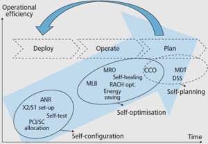
Figure 1. SON parameters as a function of network engineering cycle stages [3].

There are now numerous tools designed to simplify the tasks of inserting and planning new network elements such as those used for propagation models, automatic cell planning and automatic frequency planning. However, many of these integration and configuration tasks are performed manually. When a new base station is installed, some parameters are required, such as configuring transport links, establishing connectivity with the network core, neighborhood relations, transmission power, and others. All these stages are time-consuming, error-prone, and effort-intensive.

In consonance with self-manageable networks and reduced human intervention, the Plug and Play concept was created for SON networks. This concept refers to the ability of network elements to configure themselves automatically when installed on a network to then provide services depending on their functions. This self-configuring process uses data already found in the network, which are used for network element itself to be able to configure itself.

III.1.1 Self-configuration process

The process begins with the assignment of an IP (Internet Protocol) address using technologies such as DHCP – Dynamic Host Configuration Protocol for a newly added base station and the establishment of automatic contact with OAM (Operation and Maintenance). After that, the station is authenticated and associated with the network gateway. After connecting to the gateway, the software and parameters needed for self-configuration are downloaded and radio configuration begins for transmission power, cell identification, antenna tilt and neighborhood list configuration.

Figure 2 shows each stage of the distributed Self-Configuration process with their ramifications.

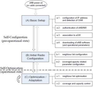
Figure 2. Self-Configuration Process [4].

A network configuration must ensure that a certain quality of service level is met when in operational mode. After making the necessary configurations, the network optimization and operation phase begins.

III.1.2 Deploying a new base station

The flowchart in Figure 6 shows the stages of deploying a new base station and the relationship of self-configuration stages with network management elements.

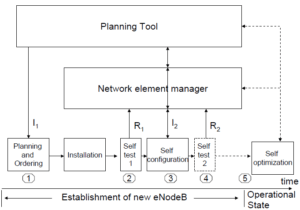
Figure3. Flowchart to deploy a new base station [5].

During the first stage, planning for the new station is based on coverage and capacity requirements, and may also reference network measurements. Initial parameters (I1) during planning may include location, antenna type, cell characteristics (sectorization) and maximum capacity [5]. Once a station has been physically installed, self testing starts with any reporting to the network manager (R1). When self-testing ends, self-configuration starts and then the station requests the basic configuration data (I2) addressed in topic III.1.1.

At the end of the procedure, the station has to report its existence to neighbors, include new cells in the neighborhood list, and configure specific neighborhood parameters in these cells.

Next, the main Self-Configuration functionalities will be described in items A, B and C below.

 A. Automatic Software Download

Através do sistema de OAM, os elementos da rede podem realizar uma verificação do software vigente e compará-lo com a versão disponibilizada pelo operador. Caso tenha sido verificada uma versão mais recente, o software é automaticamente transferido para os elementos correspondentes. Este procedimento acelera a atualização e automatiza o processo, gerando ganhos devido à instalação prévia de um software otimizado e à não necessidade de intervenção direta do operador.

B. Automatic Inventory

O Automatic Inventory possibilita, através de túneis de gerenciamento (SeGW – Security Gateway [6]), que a eNodeB forneça ao operador todas as informações referentes as alterações de hardware realizadas na rede. Sendo assim, todo e qualquer elemento adicionado à rede aparecerá automaticamente na interface de gerência do operador, não sendo necessária sua presença no local do site para realizar o reconhecimento do elemento adicionado. Para tanto, faz-se necessário que cada unidade instalada tenha consigo uma identificação, Hardware Identifier / Label, o que garante seu reconhecimento imediato, propiciando a visualização remota da rede e as consequências de cada elemento adicionado.

C. Automatic PCI Planning

PCI (Physical Cell Identification) operates on a cell’s physical layer level. This identification is unique and cannot be repeated in nearby cells. It may be thought of as the cell’s signature. There are 504 identities available to be distributed among cells. Its value is obtained using the following expression:

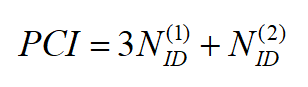
The PCI is defined by the operator using a planning tool that ensures a sufficient margin of separation between two RBSs so that there is no mutual interference between radio bases with the same PCI value.

Therefore, the operator must be careful when mapping cells and their PCIs, otherwise, there may be neighboring cells with the same PCI value in which case the mobile will be unable to discern one cell from another, thus causing a handover failure, among other problems.

Through Automatic PCI Planning, during the operational stage, each RBS collects data on any PCI related conflicts that may arise. In addition to the automation generated by the process, mobile devices collaborate by reporting to the RBS server whenever they get signals from cells with the same PCI. If there is a positive conflict, an algorithm called POT (PCI Optimization Tool is activated to collect and analyze logs generated by RBSs and mobiles, thus identifying which cells caused conflict. With these data, PCI values may be altered to end conflict.

In the case of Self-Configuration, the 3GPP – (3rd Generation Partnership Project) proposal stipulates collision-free automatic PCI configuration so there are different operating modes depending on the developer. Some advocate a decentralized solution in which RBSs are enabled to automatically configure their PCIs. Others advocate a centralized solution, in which the calculation is automated, but the final PCI assignment decision depends on the operator and is given through the OAM system [7]. Both solutions are briefly described below:

• Decentralized

Once a radio base has been installed, a random PCI will initially be used, and for a certain period of time the Automatic Neighbor Relation (ANR) function is used to collect PCI data from neighboring cells. Once data has been received from neighboring cells, it may automatically configure its own PCI value to avoid collisions. Note that this solution does not always eliminate collisions immediately because if there is a fault when receive neighboring PCIs, the radio base may be configured with a value that is already being used, so another verification would be required.

• Centralized

In this case, each installed base radio has a central function that stores data for location and PCIs adopted. Using this data and knowing its own location, the base station is able to make the necessary calculations and automatically choose a PCI value that meets 3GPP requirements.

III.2. Self-Optimization

Due to growing user numbers and heavier data traffic demand, smaller cells have to be used to leverage reuse of frequencies and enable more broadband for users. Starting from this point, one may conceive of a network with a larger number of base stations, so keeping them working optimally involves more difficulty. Managing this network along with previous technologies, may become overly complex and any inefficient performance may directly affect user experiences.

Through the use of this application, cell parameters are monitored. Based on this information, the network can make decisions in order to optimize its elements’ quality and consequently their performance, so complex or time-consuming manual tasks can now be run quickly and automatically. This makes a network flexible and highly adaptable to different usage situations [8].

Optimization techniques are among the main elements in Self-Organizing Networks, since even after installing and configuring network elements, the environment may undergo alterations, which shows that networks have to be dynamically optimized. There are several situations that alter the characteristics of a network [9]:

• Changed traffic levels

During certain periods of the day, data traffic in the same location may vary, e.g. smartphones may be used less intensively while working but more intensively during lunch breaks. In general, network traffic was heavier due to the development of technologies and widespread use of smartphones.

• Changes in physical characteristics within cell

Basic changes made to a cell’s environment, such as adding a new building, installing an outdoor billboard, or even cars and traffic, may alter propagation characteristics so signal strength within the cell’s coverage area may vary with changes in the environment.

• Deploying new services

When new services are being deployed, new radio stations will often have to be added, or a station that changes its characteristics will have to be updated.

• Major events

In areas near centers holding major events, such as football stadiums or large concert halls, radio bases with flexible characteristics are often needed in order to direct signals during events, ensuring that users in the place can all access them at the same time without any issues.

So in employing a system that automatically adapts to all changes made in a network is highly advantageous. Some improvements are noticeable, such as energy savings, automatic and dynamic adjustment of site parameters – hence higher quality service offered users.

Next, sub-items A to F contain detailed descriptions of the Self-Optimization functionalities listed in Figure 7.

A. Automatic Neighbor Relation

If mobile systems are to work harmoniously, each base station must maintain a relation with adjacent base stations. The Automatic Neighbor Relation (ANR) function enables the association between neighboring cells to be optimized, so the network operator’s physical presence is no longer needed for this process. 3G and 4G system radio bases have PCI, CGI – Cell Global Identity and ECGI – EUTRAN Cell Global identifiers and their function is mapping cells among themselves and across the entire coverage area.

Each RBS has a Neighbor Relation Table (NRT) for each cell, in which all its neighbor relationships with adjacent cells are defined. The NRT stores data for which cells will be added or removed, for which the handover should be directed and whether the X2 interface between the two eNodeBs should be created [10].

The procedure that would be followed by a network operator using planning tools is now automated due to the intervention of Self-Optimization technologies, which used measurements made by the mobile device to fill out the table without the operator’s intervention. Prediction errors may be very harmful for a network, since handover relationships depend on correctly filling the NRT so that base stations know where to transfer a mobile that is on the edge of a cell. Given the above, the planning procedure must be followed repeatedly so that cell edges are well defined as well as which relationships there may be, a practice that add to operators’ costs and highlights the need to use SON techniques.

Each neighborhood relationship that will be added to the NRT table is inserted in the Target Cell Identifier (TCI) field found in the table. For example, if the source and target cells are both from an LYTE system on the same frequency, then the TCI field assumes the target cell’s ECGI value, which is the identifier of each base radio in the entire mobile network.

Figure 8 shows the NRT filling mode for an LTE system.

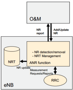
Figure 8. Filling NRT table [11].

With the advent of SON technologies, the process may be automated. Through measurements made by the mobile, coordinated by the Radio Resource Control (RRC) protocol, which establishes system access control functions, the ANR function fills the table with data on adding/removing neighbors, possibility of handover and creation of X2 interface between two eNodeBs. In short, there are two ANR models, namely:

• Intra-LTE / ANR frequency

Taking LTE as an example, the UE first makes measurements to see which cell is most powerful. If the chosen cell has an unknown PCI value (newly added cell), the server then instructs the UE to collect this cell’s ECGI and automatically adds it as a neighbor in the NRT table.

• Inter-RAT / ANR Inter-frequency

In this case, the User Equipment (UE) makes measurements and detects cells on other frequencies and other Radio Access Technologies (RATs). For Inter RAT /ANR frequency, each cell has a list showing on which frequencies the cells should be sought. The cell insertion process in the neighborhood table is very similar to the Intra-frequency modality, except for identifiers. For 4G, read ECGI and Tracking Area Code (TAC). Once measurements have been made, the server adds CGI or ECGI identifiers to the NRT table, and then the neighborhood relationship is established.

B. Load Balancing

The Load Balancing function, also known as Mobility Load Balancing (MLB), enables overloaded cells to redirect some of their traffic to adjacent less overloaded cells. Therefore the load generated by subscribers is distributed to available neighboring cells so that network capacity is maximized. This additional efficiency that is generated raises each cell’s average utilization and avoids the need to deploy more radio bases to meet user demand.

MLB algorithms can be run in two different ways:

• Distributed

Os algoritmos são executados na própria estação Rádio Base e as informações obtidas são trocadas entre as próprias estações. A interface X2 é opcional e pode ser utilizada para a comunicação entre as eNodeBs.

• Centralized

Algorithms are executed in external processing units that receive data reported by the radio bases and return data obtained through management interfaces.

The MLB becomes more robust when the users involved in the operation are in active mode, because in this case, since they are effectively using the network, they have data for the traffic generated, as well as channel conditions at that time. When there is a need for MLB for users in idle mode, the system is based on data traffic generated when they were in active mode.

Quality of Service (QoS) parameters are also used so that the system can decide how often users should reselect cells.

C. Handover Optimization

Handover Optimization consists of automating handover parameter definitions in order to make the procedure more fault-free with fewer losses for user and network. By using handover parameter control algorithms through intelligent updating of the list of neighboring cells and virtual manipulation of hysteresis parameters, any problems arising from a defective handover are substantially diminished.

There are three basic requirements defined by 3GPP for the optimization of handover parameters using SON: reduce handover failures, minimize unnecessary number of executions and increase load distribution capacity of the network’s (Load Balancing) [12].

In mobile networks without the presence of SON, the algorithms executed to initiate the exchange of cells have as main variable the signal strength received at mobile terminals. When the mobile notices the presence of a stronger signal than the current one, the handover process begins. Due to signal strength variations and the channel’s random characteristic, the effect known as “ping-pong” may occur, which consists of the mobile changing cells repeatedly, without remaining in just one. The graph in Figure 9 defines the mentioned process, in an LTE network, showing examples of measurements made by the mobile, its Reference Signal Received Power (RSRP) reception power levels and durations. The mobile is camped on eNB A, with reception power Pa.

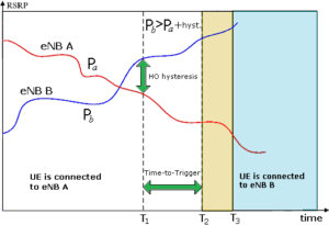
Figure 9. Handover process in an LTE network [13].

When a user is on the cell’s threshold and power higher than its current one is measured (power Pb coming from eNB B), a wait time is assumed, and the handover process is subsequently initialized.

However, to work around the “ping-pong” problem, a hysteresis is considered in order to provide a margin between the powers measured, thus preventing the mobile from returning to its station of origin. In addition to hysteresis, a time is counted until handover takes place. This time is called Time To Trigger (TTT).

When using SON, through the manipulation of hysteresis and TTT, associated with oscillation control algorithms, the unnecessary amount of cell exchange executions may be satisfactorily mitigated, thus avoiding an undesirable user experience. There is also the possibility of optimizing handover performance through algorithms based on the user mobile’s speed. In this scheme, hysteresis and TTT values are adjusted to boost handover speeds from 0 to 350 km/h, due to heavier use in transportation means using in this speed range [14].

Handover Optimization also has a positive effect on Load Balancing processes, since handover decisions are more accurate, which facilitates switching users to cells used to balance network traffic, as explained in section B.

D. Coverage & Capacity Optimization

The procedures traditionally used to alter a cell’s capacity and coverage radius are expensive and extremely complex [15]. Altering some of these characteristics requires several modifications, including the antennas’ physical aspects. In the vast majority of cases making these alterations manually is inviable therefore automated antennas had to be used. Controls could alter their inclination and several other operating parameters [16], such as the “Antenna tilt” case shown in Figure 10.

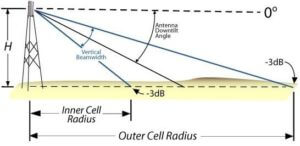
Figure 10. Antenna Tilting Function [16].

Two operations may be performed By controlling an automated antenna:

• Downtilt

Diminishes antenna angle, which reduces its coverage area.

• Uptilt 

Broadens antenna angle, thus expanding its coverage area.

This type of antenna, combined with SON technology, provides a dynamic scenario that automatically adapts to use situations, making several improvements in the network, such as:

• Reduced interference between neighboring cells

When signal interference between neighboring cells is at higher levels, the network automatically reduces the coverage area of one of the cells in order to reduce this interference.

• Optimized resource use

Traffic may be evenly distributed across the network thus optimizing signal-to-noise ratio. Therefore network capacity is raised so users may be added without losing quality of service.

• Optimized user balancing

Based on usage statistics, the network may diminish the size of a cell that has many connected users and increase the size of a neighboring cell that has a smaller number of users, in order to balance numbers of users across cells.

E. Mobility Robustness Optimization

The Mobility Robustness Optimization (MRO) function may be seen as part of the Handover Optimization process. Its main objectives are to minimize Radio Link Failure (RLF), reduce the numbers of unnecessary handovers and handovers to wrong target cells. The function includes automated detection, correction, and optimization processes, thus directly affecting good quality of service for end users while also helping to optimize energy used by the stations [17].

In order to optimize energy, some cells may be deactivated when there are no users. Energy used by base stations depends not only on whether there are active users or not, since there is a series of internal tasks that also make use of this energy. Even if the cell is powered off, there are regulations that require coverage at all times. This cell suspension takes place when the last user leaves the cell. If there is a considerable increase in network traffic, cells that remain connected and providing access may “wake up” another cell that has been suspended. They do so by sending a wake-up signal to the sleeping cell [18].

Faults that may take place in the handover process were drivers for the development of this function. Among these inaccuracies, the following stand out:

• Late Handover

In the case of Late handover, as Figure 11 shows, the cell switching process is initiated after a certain delay. In this case, the mobile is moving faster than expected for the handover procedure as the user who was initially at a certain distance from the base radio quickly starts moving further away. Therefore, the radio base sends the HO RRC handover command to initialize handover at low intensity, based on its first measurement. This transmission power is insufficient for mobile reception, because due to its speed, it is already well ahead of what the cell had been expecting by at the time of sending the command. In this case, dropped calls and data service outages are quite likely. From this point on, the mobile will reestablish its communication through a new authentication in the current cell. Subsequently, the target RBS reports the faults to the source cell in order to tune handover parameters.

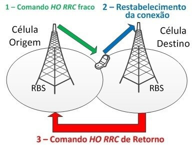
Figure 11. Late Handover.

 

• Early Handover 

Early handover as Figure 12 shows, happens when a mobile is in an intersection area between two cells, where the handover process is initiated by sending the HO RRC command to the mobile, but the signal strength level of the source cell was still enough to respond to this mobile. This scenario is often found in dense urban areas [19]. Once a handover has been completed, the mobile may detect the source cell’s signal level and find that it is better than the target cell’s, so it then triggers a new handover. This time the target cell’s RBS sends a HO RRC command to the source cell and does the return back to the previous cell.

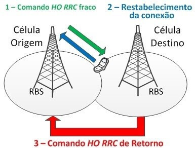
Figure 12. Early Handover.

• Handover to wrong cells

This happens when the mobile initializes the handover process then but loses its connection to the selected target RBS. When the connection has been lost, the mobile tries to reconnect to an RBS that is neither source RBS nor the target RBS. On trying to reconnect, this RBS detects a handover to the wrong cell and sends feedback to the source RBS in order to configure the handover parameters and minimize these cases.

•  Unnecessary Handovers

This may happen when handover hysteresis parameters are not properly tuned. This may cause effects such as the “ping-pong” mentioned in item C of section V.

To minimize this problem, after the handover process, the mobile device is instructed by the handover target cell to continuously measure the source cell’s signal strength level. Based on these measurements, the target cell decides whether the handover performed was done effectively, if not, it provides feedback to the source cell to tune its handover parameters.

F. Optimizing RACH

The Random-Access Channel (RACH) is used for the mobile to access the system, in which identification data and reason for access are sent. This process uses valuable network resources and so optimizing it poses considerable gains for the economic use of these resources.

While a user’s device is communicating with the network, a number of slots are allocated for RACH data, which are crucial for the system to be able to insert this user in the network. A malfunctioning access procedure causes losses such as delays when starting calls, resuming data when the mobile device switches between handover operating and delay modes.

For the access procedure to work properly, more slots must be reserved for the RACH, otherwise users may experience collisions. However, using many RACH slots is not always advantageous in terms of loss of capacity since fewer resources will be available to drain a user’s useful data. SON technologies therefore have the function of automating the operation of this procedure so that there is a compromise when choosing the number of slots reserved for RACH, assessing its real need at that time. The ideal number of reserved slots depends on the quality of service provided and the number of users in this network. Since the number of users is variable in the time domain, deciding an optimized number of resources reserved for RACH also becomes a variable in this domain [19].

In relation to delays, interference between users is also a relevant point. When a user wants access to the network, a default-power RACH preamble is first sent. If there is no response, a second attempt is made, this time at higher power, and this process continues until the mobile gets access or reaches the maximum number of increments. If the number of increments reaches its maximum value, the process starts again using minimum power and repeating the entire procedure. This procedure is adopted so that a mobile accesses the network using the lowest possible power, thus avoiding mutual interference. However, if faulty access is not due to low power but to network congestion, the mobile will continue to send preambles ay higher power levels from time to time, which obviously increases interference in the Physical Uplink Shared Channel (PUSCH) and Physical Random-Access Channel (PRACH) as in Figure 13, which shows preambles in red and other channels (PUCCH – Physical Uplink Control Channel) as a function of frequency and time slots.

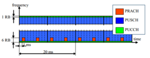
Figure 13. Physical layer random access procedure [20].

The RACH preamble sequences are derived from cyclic shifts of a Zadoff-Chu Root Sequence [21] and 64 preambles are assigned to each cell. For small cells, preambles may be derived from just one root sequence, and are orthogonal to each other. For larger cells, not all preambles are derived from the same root sequence, therefore, they may not be orthogonal, which generates a non-zero cross-correlation, generating interference between users.

If random access fails, due to not receiving the preamble from the radio base or due to collision, the mobile must start the process again. To more conflicts in this procedure, there is the Backoff parameter, which represents a time until a new access attempt is started.

To mitigate the abovementioned problems, RACH Optimization acts in the following ways:

•   In RACH configuration
  

By automatically selecting the number of RACH slots in the communication frame in order to avoid slots being occupied unnecessarily.

• Setting RACH preamble parameters

By intelligent manipulation of the backoff parameter, an optimized time to initialize access may be determined, thus avoiding congestion.

• Setting mobile power parameters

Initial power and its increments are intelligently adjusted to avoid mutual interference. Mobiles in regions where there is more fading will initialize at higher levels of power, also when they are far from the radio base. Mobiles in regions where there is less fading or mobiles camped in smaller cells, use lower levels of transmission power.

III.3. Self-Healing

Self-Healing is a set of SON procedures that detects and solves problems or simplifies them to prevent further damage to network consistency, thus significantly lowering maintenance costs. This feature is stimulated by alarms generated by network elements showing errors. In cases of reported alarms, the system collects information from tests, makes an accurate analysis and then takes appropriate measures to correct or minimize the fault’s effects.

Radio base station components are extremely susceptible to defects since as they are often exposed to a wide range of weather/climatic conditions. Any loss of service within the base station will give rise to access downtime or significantly degraded services in terms of performance. This problem may lead a loss of revenue for the operator and the possibly a higher churn rate in terms of numbers of customers cancelling their contract.

The Self-Healing application may be subdivided into a few parts. One of them is detecting cellular network degradation: performance of base stations is constantly monitored to see whether they are within acceptable limits for optimized operation.

The cellular network’s self-compensation is also an important part since its main purpose is to compensate for an adjacent cell’s inoperability. One of the essential requirements for any cellular compensation is that a network must respond quickly so that a fault is detected immediately, and its impacts are minimized. All of this process is automated. When there is a fault, the radio base searches for embedded SON algorithms to solve the problem, whatever it may be. However, this is not always possible, since the cell side fault be total, in which case compensation must come from neighboring cells.

Compensation mode widens the coverage area of neighboring stations in order to cover the location that was previously covered by the defective radio base station. On the other hand, the reuse factor of these cells is increased, so the radio base stations’ transmission power has to be boosted to get a higher signal-to-noise ratio over a large part of the cell’s area.

IV. Conclusion

Due to the high complexity of network management caused by heavier data traffic, Self-Organizing Networks have become a major trend in the mobile telephony market. Interoperability between networks using different technologies makes the mobile system dense and heterogeneous. So effective control of the entire network is required to ensure that all elements act in harmony. The above points to the inevitability of using SON, which leads to substantial improvements due to the inherent difficulty of manually configuring, operating, and healing/restoring dense networks. Automated control and management processes using SONs end the need for human intervention. This technology enables a scenario in which a network may be totally adaptable to any changed usage parameters. With this application acting on end-to-end management and control processes in a mobile phone network, volume operating expenses may be significantly mitigated, costs reduced, and user experience considerably heightened.

In addition to financial and operational benefits from using SON, operators’ customers can enjoy higher levels of reliability and better experiences since users will notice SON-optimized parameters albeit indirectly, since mobile users will see their usual activities, such as handovers, taking place more fluidly and free of faults. Higher quality service is reflected in customer satisfaction and loyalty to the operator.

V. Reference

[1] R. Estevam. Redes SON: Conceitos e aplicabilidade em redes (Outubro, 2015) Disponível em: <http://www.teleco.com.br/tutoriais/tutorialredeson/> Acesso em: 20 de julho de 2022.

[2] Operadoras buscam mais receita no pré-pago. Disponível em: <http://economia.estadao.com.br/noticias/geral,operadoras-buscam-mais-receita-no-pre-pago,387841> Acesso em: 20 de julho de 2022.

[3] L. Jorguseski et al., Self-organizing networks in 3GPP: Standardization and future trends, IEEE Communications Magazine, Communications Standards Supplement (2015).

[4] 3GPP TS 36.300 Release 13 Evolved Universal Terrestrial Radio Access Network Disponível em: <http://www.3gpp.org/ftp/specs/archive/36_series/36.300/> Acesso em: 20 de julho de 2022.

[5] 3GPP TR 32.816 Release 8 Study on management of Evolved Universal Terrestrial Radio Disponível em: http://www.3gpp.org/ftp/specs/archive/32_series/32.500/ Acesso em: 21 de julho de 2022.

[6] Wikipedia, Home eNodeB. Disponível em <https://en.wikipedia.org/wiki/Home_eNode_B> Acesso em: 22 de julho de 2022.

[7] Magdalena Nohrborg, Self-Organizing Networks. Disponível em: <http://www.3gpp.org/technologies/keywords-acronyms/105-son> Acesso em: 24 de julho de 2022.

[8] Radio-Electronics, SON Self-Optimization (Self-Optimizing Network). Disponível em: <http://www.radio-electronics.com/info/cellulartelecomms/self-organising-networks-son/self-optimisation-optimization.php> Acesso em: 24 de julho de 2022.

[9] Jae ho, Lee. SON,self-optimized network. Chapter 3. Disponível em: <http://pt.slideshare.net/gprsiva/chap-special-addition-son> Acesso em: 25 de julho de 2022.

[10] LTE World, Automatic Neighbor Relation. Disponível em: <http://lteworld.org/wiki/automatic-neighbour-relation-anr> Acesso em: 27 de julho de 2022.

[11] A. Dahlén; A. Johansson; F. Gunnarson; J. Moe; T. Rimhagen; H. Kallin. Evaluations of LTE Automatic Neighbor Relations. (2013). Disponível em: <http://www.ericsson.com/res/docs/2013/evaluations-of-lte-automatic-neighbor-relations.pdf> Acesso em: 28 de julho de 2022.

[12] Alonso-Rubio, Jose (2010, November). Self-Optimization for handovers Oscillation Control in LTE. Disponível em http://www.ericsson.com/res/thecompany/docs/journal_conference_papers/wireless_access/noms2010_HOosc.pdf Acesso em: 28 de julho de 2022.

[13] Mera, handover Parameter Optimisation in LTE. Disponível em: <https://www.mera.com/competences/mobile-networks/research/handover> Acesso em: 1 de agosto de 2022.

[14] Luan, L.; Wu, M.; Shen, J.; Ye, J.; He, X. Optimization of handovers algorithms in LTE high-speed railway networks. JDCTA (2012, June), 79–87. Disponível em: <http://www.mdpi.com/1999-5903/7/2/196/htm> Acesso em: 2 de agosto de 2022.

[15] Reverb Networks, Antenna Based Self Optimizing Networks for Coverage and Capacity Optimization (2012). 

Disponível em: <http://www.reverbnetworks.com/wp-content/uploads/2014/06/Reverb_wp_Antenna-Based-SON-for-CCO_Feb12rs.pdf> Acesso em: 2 de agosto de 2022.

[16] Proxim Wireless, Calculations: Downtilt Coverage Radius. Disponível em: <http://www.proxim.com/products/knowledge-center/calculations/calculations-downtilt-coverage-radius> Acesso em: Acesso em: 3 de agosto de 2022.

[17] GHADIALY, Zahid; Mobility Robustness Optimization To Avoid handover Failure. Disponível em: <http://blog.3g4g.co.uk/2011/07/mobility-robustness-optimization-to.html> Acesso em 20 de Abril de 2016.

[18] Basic LTE. Understanding basic concepts for LTE (September 2014). Disponível em: <http://lteshare.blogspot.com.br> Acesso em: 3 de agosto de 2022.

[19] M. Kottkamp, A.Rössler, J. Schlienz, J. Schütz. LTE Release 9 Technology Introduction (White Paper) (2010, December). Disponível em: <https://pt.scribd.com/doc/78167572/30/RACH-Optimization> Acesso em: 4 de agosto de 2022.

[20] Mehdi Amirijoo, Pål Frenger, Fredrik Gunnarsson, Johan Moe, Kristina Zetterberg. (2009). On Self-Optimization of the Random Access Procedure in 3G Long Term Evolution. Disponível em: <http://www.ericsson.com/res/thecompany/docs/journal_conference_papers/wireless_access/IM2009.pdf> Acesso em: 5 de agosto de 2022.

[21] Evolved Universal Terrestrial Radio Access (E-UTRA); Physical channels and modulation, 3GPP TS 36.211, 2015.